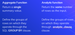
The easiest way to understand analytic functions is to start by looking at aggregate functions. An aggregate function aggregates data from several rows into a single result row.
The aggregate function reduces the number of rows returned by the query but analytical functions won’t.
select ename,deptno,teams,sal,
sum(sal) over (partition by deptno) sum_dept
from emp;
The query will return all rows of the emp table along with the department-wise sum of salary. We have not used group by clause here.
| ENAME | DEPTNO | TEAMS | SAL | sum_dept |
| MILLER | 10 | 1001 | 1300 | 22440 |
| RAINA | 10 | 1001 | 2850 | 22440 |
| SACHIN | 10 | 1001 | 1260 | 22440 |
| SEHWAG | 10 | 1002 | 2855 | 22440 |
| KING | 10 | 1002 | 5000 | 22440 |
| DHONI | 10 | 1002 | 1250 | 22440 |
| CLARK | 10 | 1002 | 2500 | 22440 |
| ROHIT | 10 | 1002 | 2450 | 22440 |
| VIRAT | 10 | 1002 | 2975 | 22440 |
| FORD | 20 | 2001 | 3100 | 25350 |
| ADAMS | 20 | 2001 | 1100 | 25350 |
| SCOTT | 20 | 2001 | 3000 | 25350 |
| JONES | 20 | 2002 | 2750 | 25350 |
| SMITH | 20 | 2002 | 800 | 25350 |
| FINCH | 20 | 2003 | 1500 | 25350 |
| STARC | 20 | 2003 | 1550 | 25350 |
| PONTING | 20 | 2003 | 6000 | 25350 |
| CLERK | 20 | 2003 | 2900 | 25350 |
| WARNER | 20 | 2004 | 2650 | 25350 |
Consider another example.
select ename,deptno,teams,sal,
sum(sal) over (partition by deptno,teams) sum_teams
from emp;
Here we are going to see the team-wise (Within the department) sum of salary.
| ENAME | DEPTNO | TEAMS | SAL | sum_teams |
| SACHIN | 10 | 1001 | 1260 | 5410 |
| RAINA | 10 | 1001 | 2850 | 5410 |
| MILLER | 10 | 1001 | 1300 | 5410 |
| DHONI | 10 | 1002 | 1250 | 17030 |
| ROHIT | 10 | 1002 | 2450 | 17030 |
| SEHWAG | 10 | 1002 | 2855 | 17030 |
| CLARK | 10 | 1002 | 2500 | 17030 |
| VIRAT | 10 | 1002 | 2975 | 17030 |
| KING | 10 | 1002 | 5000 | 17030 |
| FORD | 20 | 2001 | 3100 | 7200 |
| ADAMS | 20 | 2001 | 1100 | 7200 |
| SCOTT | 20 | 2001 | 3000 | 7200 |
| SMITH | 20 | 2002 | 800 | 3550 |
| JONES | 20 | 2002 | 2750 | 3550 |
| FINCH | 20 | 2003 | 1500 | 11950 |
| STARC | 20 | 2003 | 1550 | 11950 |
| PONTING | 20 | 2003 | 6000 | 11950 |
| CLERK | 20 | 2003 | 2900 | 11950 |
| WARNER | 20 | 2004 | 2650 | 2650 |
Syntax and Examples
analytic_function([ arguments ]) OVER (analytic_clause)
The analytic_clause is divided into the following optional elements.
[ query_partition_clause ] [ order_by_clause [ windowing_clause ] ]
Eg:- select ename,deptno,teams,sal,sum(sal) over (partition by deptno order by sal rows between unbounded preceding and current row) sum_deptfrom emp;
The order_by_clause is used to order rows within the partition.
So if an analytic function is sensitive to the order of the rows in a partition you should include an order_by_clause.
Eg:
SELECT empno, deptno, sal, FIRST_VALUE(sal IGNORE NULLS) OVER (PARTITION BY deptno ORDER BY sal ASC NULLS LAST) AS first_val_in_dept FROM emp;
- Windowing_clause gives analytic functions a further degree of control within the current partition,
- It considers a whole result set if no partitioning clause is used.
- The windowing_clause is an extension of the order_by_clause and as such, it can only be used if an order_by_clause is present. The windowing_clause has two basic forms.
- RANGE BETWEEN start_point AND end_point
- ROWS BETWEEN start_point AND end_point
- RANGE BETWEEN start_point AND end_point
A specific number of rows relative to the current row.
- ROWS BETWEEN start_point AND end_point
Specify the range of values for a specific column relative to the value in the current row.
Possible values for start_point and end_point
- UNBOUNDED PRECEDING: Start from the first row of the partition, if there is no partition start from the first record.
- UNBOUNDED FOLLOWING: End at the last row of the partition, if there is no partition ends at the last record.
- CURRENT ROW: Start and end at current row.
- VALUE PRECEDING: A logical offset for the start point of RANGE_BETWEEN or A specific value for the start point of the ROWS_BETWEEN.
- VALUE FOLLOWING: Like above, But it is after the current row